Why are machine learning algorithms hard to tune?
In machine learning, linear combinations of losses are all over the place. In fact, they are commonly used as the standard approach, despite that they are a perilous area full of dicey pitfalls. Especially regarding how these linear combinations make your algorithm hard to tune.
Therefore, in this post we hope to lay out the following arguments:
- A lot of problems in machine learning should be treated as multi-objective problems, while they currently are not.
- This lack of multi-objective treatment leads to difficulties in tuning the hyper-parameters for these machine learning algorithms.
- It is nigh on impossible to detect when these problems are occurring, making it tricky to work around them.
- There are methods to solve this which might be slightly involved, but do not require more than a few lines of code. One of these methods is laid out in a follow-up blog post.
Nothing of this article is novel. You might already be aware of everything we wanted to say. However, we have the impression that most machine learning curricula do not discuss optimisation methods very well (I know mine did not), and consequently, gradient descent is being treated as the one method to solve all problems. And the general message is that if an algorithm does not work for your problem, you need to spend more time tuning the hyper-parameters to your problem.
In the next blog post, a solution is introduced, based on the NIPS’88 paper which introduced the Modified Differential Method of Multipliers.
So we hope that this blogpost can remove some confusion on how to handle this issue in a more foundational and principled way. And hey, maybe it can make you spend less time tuning your algorithms, and more time making research progress.
Linear combinations of losses are everywhere
While there are single-objective problems, it is common for these objectives to be given additional regularisation. We have picked a selection of such optimisation objectives from across the field of machine learning field.
First off, we have the regularisers, weight decay and lasso. It is obvious that when you add these regularisations, you effectively have created a multi-objective loss for your problem. After all, what you really care about, is that both the original loss \(L_0\) and the regulariser loss are kept low. And you will tune the balance between the two using a \(\lambda\) parameter.
$$ L(\theta) = L_0(\theta) + \lambda \sum \left| \theta \right| $$
$$ L(\theta) = L_0(\theta) + \lambda \sum \theta^2 $$
As a consequence, losses found in e.g. VAE’s are effectively multi-objective, with a first objective to maximally cover the data, and a second objective to stay close to the prior distribution. In this case, occasionally KL annealing is used to introduce a tunable parameter \(\beta\) to help handle the multi-objectiveness of this loss.
$$ L(\theta) =\mathbb{E}_{q_{\phi}(z | x )} \left[ \log p_\theta ( x | z) \right] - \beta D_{KL} \left( q_\phi ( z | x) \| p(z) \right) $$
Also in reinforcement learning, you can see this multi-objectiveness. Not only is it common for many environments to simply sum rewards received for obtaining partial goals. The policy loss is usually also a linear combination of losses. Take as an example here the losses on the policy for PPO, SAC and MPO, entropy regularized methods with their tunable parameter α.
$$ L(\pi) = - \sum_t \mathbb{E}_{(s_t, a_t)} \left[ r(s_t, a_t) + \alpha \mathcal{H}(\cdot , s_t)\right]$$
$$ L(\pi) = - \sum_t \mathbb{E}_{(s_t, a_t)} \left[ \mathbb{E}_\pi\left(Q(s_t, a_t)\right) - \alpha D_{KL} \left( q \| \pi \right) \right]$$
Finally, the GAN-loss is of course a sum between the discriminator and the generator loss:
$$ L(\theta) = - \mathbb{E}_x \left[ \log D_\theta(x)\right] - \mathbb{E}_z \left[ \log ( 1- D_\theta(G_\theta(z))\right]$$
All of these losses have something in common, they are effectively trying to optimise for multiple objectives simultaneously, and argue that the optimum is found in balancing these often contradicting forces. In some cases, the sum is more ad hoc and a hyper-parameter is introduced to weigh the parts against each other. In some cases, there are clear theoretical foundations on why the losses are combined this way, and no hyper-parameter is used for tuning the balance between the parts.
In this post, we hope to show you this approach of combining losses may sound appealing, but that this linear combination is actually precarious and treacherous. The balancing act is often more like a tightrope walk.
Our toy example
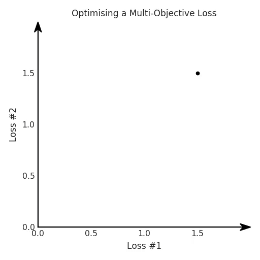
Let us consider a simple case, where we are trying to optimise for such a linear combination of losses. We take the approach of optimising the total loss, which is a sum of losses. We optimise this with gradient descent, and we observe the following behaviour.
Our code in Jax would look something like this:
def loss(θ):
  return loss_1(θ) + loss_2(θ)
loss_derivative = grad(loss)
for gradient_step in range(200):
  gradient = loss_derivative(θ)
  θ = θ - 0.02 * gradient
As is usually the case, we are not immediately happy about the tradeoff between the two losses. So we introduce a scaling coefficient α on the second loss and run the following code:
def loss(θ, α):
  return loss_1(θ) + α*loss_2(θ)
loss_derivative = grad(loss)
for gradient_step in range(200):
  gradient = loss_derivative(θ, α=0.5)
  θ = θ - 0.02 * gradient
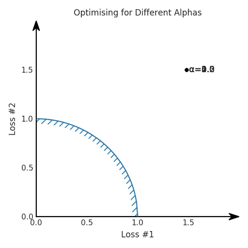
The behaviour we hope to see is that when tuning this α, we can choose the trade-off between the two losses and select the point we are most happy with for our application. We effectively will go on a hyper-parameter tuning loop, manually select an α, run the optimisation process, decide we would like the second loss to be lower, tune our α up accordingly and repeat the whole optimisation process. After several iterations, we settle for the solution we found and continue writing our papers.
However, that is not what is always happening. The actual behaviour we sometimes observe for our problem looks like the one below.

It seems that no matter how we finetune our α-parameter, we cannot make a good trade-off between our two losses.
We see two clusters of solutions, one where the first loss is ignored, and one where the second loss is ignored. However, both of these solutions are not useful for most applications. Most of the time, a point where the two losses were more balanced is a more preferred solution.
In fact, this diagram of the two losses over the course of training is barely ever plotted, so the dynamics illustrated in this figure often goes unobserved. We just look at the training curve plotting the total loss, and we might conclude that this hyper-parameter needs more time tuning, as it seems to be really sensitive. Alternatively, we could settle for an approach of early stopping to make the numbers in the paper work. After all, reviewers love data efficiency.
Where did it go wrong though? Why does this method sometimes work, and why does it sometimes fail to give you a tunable parameter? For that, we need to look deeper into the difference between the two figures.
Both figures are generated for the same problem, using the same losses and are optimising these losses using the same optimisation method. So none of these aspects are to blame for the difference. The thing which has changed between these problems is the model. In other words, the effect the model parameters θ have on the output of the model is different.
Therefore, let us cheat and visualise something which is normally not visualisable, the Pareto front for both of our optimisations. This is the set of all solutions achievable by our model, which are not dominated by any other solution. In other words, it is the set of achievable losses, where there is no point where all of the losses are better. No matter how you choose to trade off between the two losses, your preferred solution always lies on the Pareto front. By tuning the hyper-parameter of your loss, you usually hope to merely find a different point on that same front.

The difference between the two Pareto fronts is what is causing the tuning to turn out well for the first case, but to fail horribly after changing our model. It turns out that when the Pareto front is convex, we can achieve all possible trade-offs by tuning our α-parameter. However, when the Pareto front is concave, that approach does not seem to work well anymore.
Why does gradient descent optimisation fail for concave Pareto fronts?
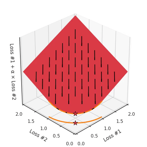
We can illustrate why that is the case, by looking at the total loss in the third dimension, the loss which is actually optimised with gradient descent. In the following figure, we visualise the plane of total loss in relation to each of the losses. While we actually descend on this plane using the gradient with respect to the parameters, each gradient descent step we take will also necessarily go downwards on this plane. You can imagine the gradient descent optimisation process as putting a spherical pebble on that plane, letting it wobble down under gravity and wait until it comes to a halt.
The point where the optimisation process halts is the result of the optimisation process, here indicated by a star. As you can see in the following figure, no matter how you wobble down the plane, you will always end up in the optimum.

By tuning α, this space stays a plane. After all, by changing α, we are only changing the tilt of this plane. As you can see, in the convex case any solution on the Pareto curve can be achieved by tuning α. A little more α pulls the star to the left, a little less α pushes the star to the right. Every starting point of the optimisation process will converge on the same solution, and that is true for all values of α.
However, if we take a look at the differently modeled problem with a concave Pareto front, it becomes apparent where our problem is coming from.
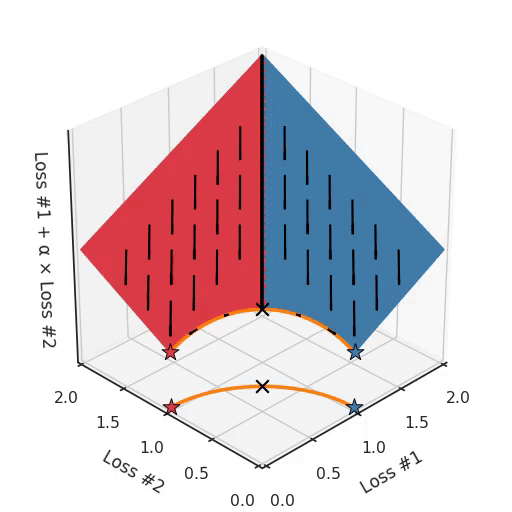
If we imagine our pebble following the gradients on this plane: sometimes rolling more to the left, sometimes more to the right, but always rolling downwards. Then it is clear it will end up in one of the two corner points, either the red star or the blue star. When we tune α, our plane is tilting in exactly the same way as in the convex case, but because of the shape of the Pareto front, only two points on that front will ever be reached, namely the points on the ends of the concave curve. The \(\times\)-point on the curve, the one which you would actually want to reach, cannot be found with gradient descent based methods. Why? Because it is a saddle point.
Also important to note is what happens when we tune α. We can observe that we tune how many of the starting points end up in one solution versus the other, but we cannot tune to find other solutions on the Pareto front.
What kinds of problems do these linear combinations cause?
To conclude this blog post, we would like to enlist the problems with using this linear combination of losses approach:
- First off, even if you do not introduce a hyper-parameter to weigh off between the losses, it is not correct to say that gradient descent will try to balance between counteracting forces. Depending on the solutions which are achievable by your model, it may very well completely ignore one of the losses to focus on the other or vice versa, depending on where you initialised the model.
- Second, even when a hyper-parameter is introduced, this hyper-parameter is tuned on a try-and-see basis. You run a complete optimisation process, decide if you are happy, and then finetune your hyper-parameter. You repeat this optimisation loop until you are happy with the performance. It is a wasteful and laborious approach, usually involving multiple iterations of running gradient descent.
- Thirdly, the hyper-parameter cannot tune for all optima. No matter how much you tune and keep fine-tuning, you will not find the intermediate solutions you might be interested in. Not because they do not exist, as they most certainly do, but because a poor approach was chosen for combining these losses.
- Fourthly, it is important to stress that for practical applications, it is always unknown whether the Pareto front is convex and therefore whether these loss weights are tunable. Whether they are good hyper-parameters depends on how your model is parameterised, and how this affects the Pareto curve. However, it is impossible to visualise or analyse the Pareto curve for any practical application. Visualising it is considerably more difficult than our original optimisation problem. So if a problem has occurred, it would go unnoticed.
- Finally, if you would really like to use those linear weights to find trade-offs, you need an explicit proof that the whole Pareto curve is convex for the specific model in use. So using a loss which is convex with respect to the output of your model, is not enough to avoid the problem. If your parametrisation space is large, which is always the case if your optimisation involves weights inside a neural network, you can forget about attempting such a proof. It is important to stress that showing convexity of the Pareto curve for these losses based on some intermediate latents is not sufficient to show you have a tunable parameter. The convexity really needs to depend on the parameter space, and what the Pareto front of the achievable solutions looks like.
Note that in most applications, Pareto fronts are not either convex or concave, but they are a mix of both. This amplifies the problem.
Note that in most applications, Pareto fronts are not either convex or concave, but they are a mix of both. This amplifies the problem. Take for example a Pareto front, where there are concave pieces between convex pieces. Not only will each concave piece make sure that none of its solutions can be found with gradient descent, it will also split the space of parameter initialisations into two parts, one which will find solutions on the convex piece on one side, and one that will only find solutions on the other. Having more than one concave piece in the Pareto front compounds the problem, as illustrated in the figure below.
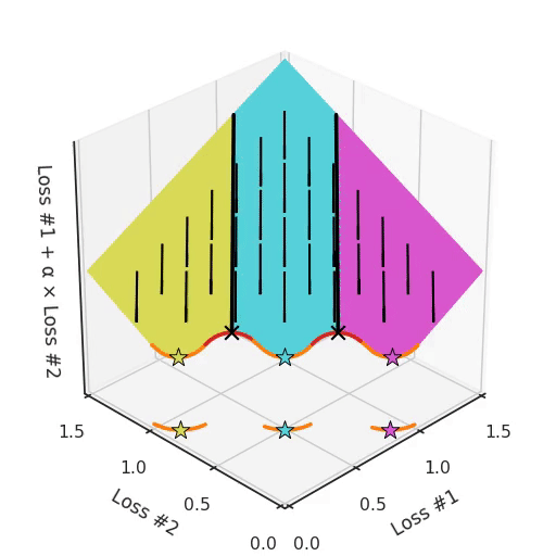
So not only do we have a hyper-parameter α which cannot find all solutions, depending on the initialisation it might find a different convex part of the Pareto curve. To make things even harder to work with, this parameter and the initialisation mix with each other in confusing ways. If you tune your parameter slightly hoping to move the optimum slightly, you can suddenly jump to a different convex part of the Pareto front, even when keeping the initialisation the same.
All of these issues do not need to be the case. There are excellent ways to deal with this issue, ways that could make our lives easier by making our optimisations spit out better solutions even on the first attempt.
In the next blog post, we detail one of these solutions based on an old NIPS’88 paper. Meanwhile, this is our first blogpost of 2021. It would mean the world to us if you could leave a comment below, and let us know if this helped you learn something new or whether we should write more of these.

